The notion of a rate of change is central to mathematics and its applications. Roughly speaking, a rate of change tells us how fast and in what manner a given quantity is changing with respect to another changing quantity. We will consider three examples below.
Suppose that a population of a town grows by \(200\) people each year. Here, the rate of change of the population with respect to time is constant and equal to \(200\) people/year.
Recall Example 1.1.6. A daily pediatric dose of Amoxicillin, \(D\text{,}\) in milligrams, depends on the weight of a patient, \(w\text{,}\) in kilograms. More precisely, \(D=50w\text{.}\) How fast does the dose increase as the weight increases? The formula for \(D\) clearly shows that for each 1 kilogram increase in weight, the dose increases by 50 milligrams. In this case, the rate of change of \(D\) with respect to weight \(w\) is \(50\) milligrams/kilogram.
Suppose that the value of your car changes at the rate \(-1500\) dollars/year. The rate of change is negative, meaning that the value of the car decreases by \(1500\) dollars each year. In general, a quantity that changes at a negative rate is decreasing while one that changes at a positive rate is increasing.
In the three examples above, the rate of change of the dependent variable with respect to the independent variable is constant. In real-life processes, this is rarely the case.
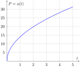
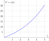
Consider the following example of two students, Amir and Nick, who went to the library to study for a precalculus exam. After \(t\) hours of uninterrupted study, Amir mastered \(P=a(t)\) pages of new material from the textbook while Nick mastered \(P=n(t)\) pages. The graphs of the two functions \(a(t)\) and \(n(t)\) are in Figure 1.5.1.
According to the graphs, both students stayed in the library for 5 hours. We can see that during the 5-hour session, both students learned about 30 new pages, as \(a(5)\approx 30\) and \(n(5)\approx 30\text{.}\)
This means that Amir went from learning quickly at the beginning of the study session to learning more slowly as time went on. Nick, on the other hand, got off to a slow start but picked up the pace as time went on. Their learning patterns are clearly not identical.
Does it make sense to ask how quickly—or at what rate in pages per hour—each student learned during the 5-hour session? Not really. The question is ambiguous. When exactly in the study session should we focus on? The beginning? The end? For both students, the rate at which they were learning during the session changed, with Amir learning more and more slowly over time and Nick learning faster and faster.
What does make sense is to consider how quickly each student learned during the 5-hour session on average. Amir learned quickly at first and then more slowly later, but overall he mastered 30 pages of new material in 5 hours. He learned at an average rate of \(\frac{30}{5}=6\) pages/hour. Nick, on the other hand, learned slowly at first, then faster, but he also mastered 30 pages in 5 hours. So, he too learned at an average rate of \(\frac{30}{5}=6\) pages/hour.
Readers who proceed to Calculus will study instantaneous rate of change—how quickly a quantity changes at a specific input. For now, the average rate of change is the best we can do.
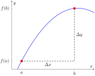
Let \(y\) be a function of \(x\text{,}\)\(y=f(x)\text{.}\) Let \(x=a\) and \(x=b\) be given. The average rate of change of \(y\) between \(x=a\) and \(x=b\) is given by
\begin{equation*}
\aroc = \dfrac{\text{Change in } y}{\text{Change in } x}=\dfrac{\Delta y}{\Delta x}=\dfrac{f(b)-f(a)}{b-a}.
\end{equation*}
Typically, the symbol \(\Delta\) (the Greek letter Delta) is used to mean “change in.” So, \(\Delta y\) stands for a change in \(y\) while \(\Delta x\) stands for a change in \(x\text{.}\) In the definition above, \(\Delta x\) stands for the change in \(x\) between \(x=a\) and \(x=b\text{.}\) This can be thought of as the distance between the numbers \(a\) and \(b\text{,}\) which is given by \(\Delta x=b-a\text{.}\) The notation \(\Delta y\) stands for the change in \(y=f(x)\) that takes place as \(x\) changes from \(x=a\) to \(x=b\text{.}\) That change is given by \(\Delta y=f(b)-f(a)\text{.}\) The graph below illustrates the changes in \(x\) and \(y\text{.}\)
This is not an applied example so \(x\) and \(y\) don’t have real-life units. In general, the average rate of change \(\dfrac{\Delta y}{\Delta x}\) is measured in
\begin{equation*}
\text{units of }\aroc = \frac{\text{units for } y}{\text{unit for } x}
\end{equation*}
Were units associated with \(x\) and \(y\) in the last example, we would write that the average rate of change of \(y\) between \(x=1\) and \(x=3\) is \(4 \; \frac{\text{units for } y}{\text{units for } x}\text{.}\)
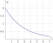
The amount of nicotine in a person’s bloodstream, \(N = f (t)\text{,}\) in milligrams, is a function of the time \(t\text{,}\) in hours, that has passed since the person smoked a single cigarette. The graph of the function \(f(t)\) is shown below.
To find the average rate of change between \(t=0\) and \(t=4\text{,}\) we use the graph to find the values of the function \(f(t)\) at \(t=0\) and at \(t=4\text{.}\) At \(t=0\text{,}\) we have \(N=f(0) = 2\) milligrams. At \(t=4\text{,}\)\(N = f(4)= 0.5\) milligrams. Thus:
Here the variables are associated with units: \(N\) is measured in milligrams while \(t\) is measured in hours. Hence, \(\Delta N\) is measured in milligrams and \(\Delta t\) is measured in hours. The average rate of change has units \(\frac{\text{milligrams}}{\text{hour}}\) which can be written as \(\frac{\text{mg}}{\text{hr}}\text{.}\)
The rate is negative as the amount of nicotine decreased between \(t=0\) and \(t=4\text{.}\) For the interpretation, we would say that on the interval \(0\leq t \leq 4\text{,}\) nicotine leaves the body at the average rate of \(0.375\) milligrams per hour.
A population \(P\) of a small village at time \(t\text{,}\) measured in years since the year 2010, is given by \(P=P(t)\text{.}\) Here are the annual readings:
The change in \(P\) between \(t=2\) and \(t=6\text{,}\)\(\Delta P\text{,}\) tells us by how much the population changed from \(t=2\) and \(t=6\text{:}\)
A ball is dropped from the rooftop of a building 150 feet tall. The height of the ball above the ground, \(h(t)\text{,}\) in feet, \(t\) seconds after the ball is dropped is:
This can also be thought of as the average velocity of the ball between \(t=0\) and \(t=2\text{.}\) The velocity is negative because the height is decreasing.
Mathematically, we get two solutions: \(t=\sqrt{9.375}\) and \(t=-\sqrt{9.375}\text{.}\) However, only one makes sense in the applied context for our problem. As \(t\) is the number of seconds after the ball is dropped, a negative answer does not make sense—the ball can’t hit the ground before it was dropped! Hence, the ball hits the ground \(t=\sqrt{9.375}\approx 3.062\) seconds after it is dropped.
In Exercise 1.3.8, data about the world population, in billions, between the years 2010 and 2018, was given in the table shown below. Use the data to answer the following questions.
What was the average rate of change of the world population between 2010 and 2012? Between 2016 and 2018? Give your answers to four decimal places and include units with your answers.
A ball is dropped from a cliff above a lake. The ball’s height above the surface of the lake, \(h(t)\text{,}\) in feet, \(t\) seconds after the ball is dropped, is given by
What is the average rate of change in height \(h(t)\) between \(t=0\) and \(t=3\text{?}\) Between \(t=1\) and \(t=4\text{?}\) Give units with your answers.
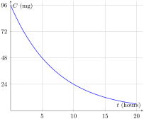
Recall that this graph that models the amount of caffeine, in milligrams, remaining in the body \(t\) hours after drinking a cup of coffee. Use the graph to do the following.
The average rate of change from \(t = 0\) to \(t = 5\) hours is larger than the average rate of change from \(t=10\) to \(t=15\) hours. It can be seen that the rate at which the amount of caffeine in the bloodstream is changing gets smaller and smaller as time progresses.
A person’s weight, \(W\text{,}\) in pounds, depends on the number of minutes \(m\) of daily exercise. Hence, \(W=W(m)\) is a function of \(m\text{.}\) Below is a numerical representation of \(W(m)\text{:}\)
Yes. From 2009 to 2010 is the only two consecutive years for which the sales increased. Therefore, this is the only one-year interval for which the ARC was positive.