Power Functions: Fractional and Negative Integral Exponents

Section 4.4 Power Functions: Fractional and Negative Integral Exponents

Objectives

After completing this section, you should be able to do the following.

First objective.
🔗

🔗
Second objective.
🔗

🔗
Third objective.
🔗

🔗

In the previous section, we considered power functions $f(x) = kx^p$ in the case when $p$ is a positive integer. When $p$ is a negative integer, power functions behave quite differently.

🔗

Subsection Negative Integral Exponents

Consider a power function

\begin{equation*} f(x) = kx^p \end{equation*}

in the case when the exponent $p$ is a negative integer. The behavior and graphs of such functions are very different from the behavior of power functions for positive integral exponents.

🔗

A negative exponent $x^{-m}$ means the reciprocal $\frac{1}{x^m}\text{.}$ So now the independent variable is in the denominator. The domain of a power function in this case is no longer the set of all real numbers as $x$ cannot be $0\text{.}$

🔗

As we will soon see, the graphs of power functions with exponents that are negative integers look very differently than in the case of positive integral exponents.

🔗

Example 4.4.1.

Which of the functions below are power functions? Rewrite those which are in standard form $y = kx^p\text{.}$ Identify the coefficient and the exponent.

🔗

$\displaystyle \displaystyle f(x) = \frac{3x^2}{2x^3}$
🔗

🔗
$\displaystyle \displaystyle g(x) = \frac{-\pi}{x^4}$
🔗

🔗
$\displaystyle \displaystyle h(x) = \frac{70}{3^x}$
🔗

🔗

🔗

Solution.

The function $f(x)$ is a power function. Using Rules of Exponents from Section 4.1, we can rewrite:

\begin{equation*} f(x) = \frac{3x^2}{2x^3} = \frac{3}{2x} = \frac{3}{2} \cdot \frac{1}{x} = \frac{3}{2} \cdot x^{-1}. \end{equation*}

The coefficient is $k = \frac{3}{2}$ and the exponent is $p = -1\text{.}$

🔗

🔗
$g(x)$ is a power function:

\begin{equation*} g(x) = \frac{-\pi}{x^4} = -\pi x^{-4}. \end{equation*}

The coefficient is $k = -\pi$ and the exponent is $p = -4\text{.}$

🔗

🔗
$h(x)$ is not a power function. Using rules of exponents for arbitrary exponents, we can rewrite:

\begin{equation*} h(x) = \frac{70}{3^x} = 70 \cdot 3^{-x}. \end{equation*}

The function $h(x) = 70 \cdot 3^{-x}$ is not a power function. Indeed, the base of the power expression $3^{-x}$ is constant at $3\text{,}$ meanwhile the exponent $-x$ varies.

🔗

🔗

🔗

Example 4.4.2.

Body mass index (BMI) is an easy screening method for weight category — underweight, healthy weight, overweight, and obesity. BMI is calculated as follows:

\begin{equation*} \text{BMI} = \frac{\text{(weight in lb)} \cdot 703}{(\text{height in inches})^2} \end{equation*}

🔗

A person who weighs 170 lb may be underweight or obese—it depends on the person’s height. Let $I(h)$ denote body mass index of a person who weighs 170 lb and whose height is $h\text{.}$ Then, according to the formula,

\begin{equation*} I(h) = \frac{170 \cdot 703}{h^2} \end{equation*}

Note that with the weight fixed at 170 lb, body mass index is a power function of height: $\displaystyle I = 119510 \cdot h^{-2}\text{.}$ (In terms of proportionality, BMI is inversely proportional to the square of height.) The obese category is defined as BMI of 30.0 or above. The normal weight category corresponds to BMI between 18.5 and 24.9.

🔗

Find the height $h$ at and below which a person weighing 170 lb is obese.

🔗

Solution.

We want to find $h$ such that $I(h) = 30\text{:}$

\begin{equation*} \frac{170 \cdot 703}{h^2} = 30 \end{equation*}

After multiplying both sides by $h^2$ and dividing by 30, then

\begin{equation*} h^2 = \frac{170 \cdot 703}{30} \end{equation*}

which gives:

\begin{equation*} h = \pm\sqrt{\frac{170 \cdot 703}{30}} \end{equation*}

Since $h$ in our problem has to be positive, the solution is:

\begin{equation*} h = \sqrt{\frac{170 \cdot 703}{30}} \approx 63 \end{equation*}

At the height $h = 63$ inches and below a person weighing 170 lb is obese.

🔗

Note that when $h$ increases $I(h)$ decreases as the denominator of the expression $\displaystyle \frac{170 \cdot 703}{h^2}$ becomes larger. On the other hand, when $h$ gets smaller, $I(h)$ gets larger. Hence, every person shorter than $63$ inches who weighs 170 lb is also obese.

🔗

Subsection Graphs of Power Functions: Negative Integral Exponents

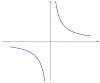
Graphs of power functions $y = kx^p$ with exponents $p$ that are negative integers have a different shape depending on whether $p$ is even or $p$ is odd.

🔗

Odd Negative Exponents

🔗

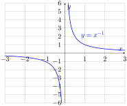
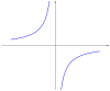
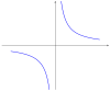
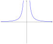
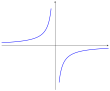
Let’s begin with the case $k = 1$ and $p = -1\text{.}$ The graph of the function $\displaystyle y = x^{-1} = \frac{1}{x}$ looks as follows:

🔗

$A short description.$

Observe that when $x$ gets larger and larger, say:

\begin{equation*} x = 1, \hspace{2pt} 2, \hspace{2pt} 3, \hspace{2pt} 4, \hspace{2pt} 5, \hspace{2pt} \dots 1000 \hspace{2pt} \dots, \end{equation*}

the values $\displaystyle y = \frac{1}{x}$ become very close to 0. Indeed, they are:

\begin{equation*} y = 1, \hspace{2pt} \frac{1}{2}, \hspace{2pt} \frac{1}{3}, \hspace{2pt} \frac{1}{4}, \hspace{2pt} \frac{1}{5}, \hspace{2pt} \dots\frac{1}{1000}\dots. \end{equation*}

🔗

In terms of the graph, this behavior translates to the graph getting very close, arbitrarily close, to the $x$-axis. We say that the $x$-axis, or equivalently the horizontal line $y = 0\text{,}$ is a horizontal asymptote of the function $y = \dfrac{1}{x}\text{.}$

🔗

Observe that as $x$ is getting close to 0 from the right, the values are becoming very large. Let’s test a few positive inputs close to 0:

\begin{equation*} x = \frac{1}{2}, \hspace{2pt} \frac{1}{3}, \hspace{2pt} \frac{1}{4}, \hspace{2pt} \frac{1}{5}, \hspace{2pt} \dots \frac{1}{1000}\dots \end{equation*}

The corresponding values $\displaystyle y = \frac{1}{x}$ are:

\begin{equation*} y = 2, \hspace{2pt} 3, \hspace{2pt} 4, \hspace{2pt} 5, \hspace{2pt} \dots 1000 \hspace{2pt} \dots \end{equation*}

In terms of the graph, this behavior translates to the graph getting very close to the $y$-axis with the values of the function becoming arbitrarily large. We say that the $y$-axis, or equivalently the vertical line $x = 0\text{,}$ is a vertical asymptote of the function $\displaystyle y = \frac{1}{x}\text{.}$

🔗

The portion of the graph corresponding to negative inputs $x\text{,}$ is symmetric about the origin to the portion of the graph corresponding to positive inputs. Indeed, when $x$ changes sign $y = \frac{1}{x}$ changes sign:

\begin{equation*} \frac{1}{-x} = -\frac{1}{x}. \end{equation*}

🔗

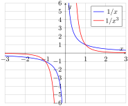
Graphs of other power functions $y = kx^p$ in which the exponent $p$ is an odd negative integer have a similar shape to the graph of $\displaystyle y = \frac{1}{x}\text{.}$ For example:

🔗

$A short description.$

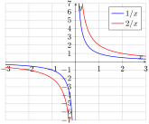
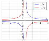
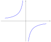
As always, the coefficient $k$ in $y = kx^p$ stretches or shrinks the graph of $y = x^p$ vertically. Additionally, if $k$ is negative, the graph is reflected about the $x$-axis.

🔗

$A short description.$

Even Negative Exponents

🔗

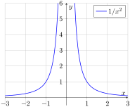
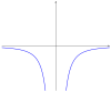
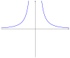
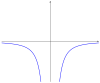
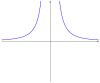
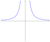
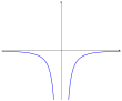
When $p$ is a negative even integer, the graph of $y = x^p$ is entirely above the $x$-axis and it is symmetric about the $y$-axis, since $(-x)^p = x^p$ when $p$ is even.

🔗

$A short description.$

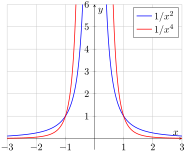
The graphs of the functions $y = x^p$ for other even negative integers $p$ have a similar shape:

🔗

$A short description.$

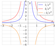
The $x$-axis is still a horizontal asymptote and the $y$-axis is a vertical asymptote. The coefficient $k$ is responsible for vertical scaling and a reflection about the $x$-axis if $k$ is negative. For example:

🔗

$A short description.$

Summary

🔗

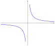
Here is a summary of how graphs of power functions look for negative integer exponents $p\text{,}$ even and odd, and for coefficients $k$ positive and negative.

🔗

$f(x)=kx^p$

🔗

$p$ even and negative

🔗

$p$ odd and negative

🔗

Positive coefficient, $k \gt 0$

🔗

$Graph of a representative power function with even negative exponent and positive coefficient.$

$Graph of a representative power function with odd negative exponent and positive coefficient.$

Negative coefficient, $k \lt 0$

🔗

$Graph of a representative power function with even negative exponent and negative coefficient.$

$Graph of a representative power function with odd negative exponent and negative coefficient.$

🔗

Subsection Fractional Exponents

Example 4.4.3.

Which of the functions below are power functions? Those which are, rewrite in standard form $y = kx^p\text{.}$ Identify the coefficient and the exponent.

🔗

$\displaystyle \displaystyle f(x) = \frac{3x^3}{7\sqrt{x}}$
🔗

🔗
$\displaystyle \displaystyle g(x) = \frac{2x^{1/3}}{x^4}$
🔗

🔗
$\displaystyle \displaystyle h(x) = \sqrt{\frac{2x}{x^{-2}}}$
🔗

🔗

🔗

Solution.

The function $f(x)$ is a power function. Using rules of exponents for arbitrary exponents, we can rewrite:

\begin{equation*} f(x) = \frac{3x^3}{7\sqrt{x}} = \frac{3x^3}{7x^{1/2}} = \frac{3x^{5/2}}{7} = \frac{3}{7}x^{\frac{5}{2}} \end{equation*}

The coefficient is $k = \frac{3}{7}$ and the exponent is $p = \frac{5}{2}\text{.}$

🔗

🔗
$g(x)$ is a power function:

\begin{equation*} g(x) = \frac{2x^{1/3}}{x^4} = 2x^{\frac{1}{3} - 4} = 2x^{-\frac{11}{3}} \end{equation*}

The coefficient is $k = 2$ and the exponent is $p = -\frac{11}{3}\text{.}$

🔗

🔗
$h(x)$ is a power function as well. Using rules of exponents for arbitrary exponents and properties of the square root, we can rewrite:
🔗

\begin{align*} h(x) \amp = \sqrt{\frac{2x}{x^{-2}}} = \frac{\sqrt{2x}}{\sqrt{x^{-2}}} = \frac{\sqrt{2} \cdot x^{1/2}}{(x^{-2})^{1/2}} \\ \amp= \frac{\sqrt{2} \cdot x^{1/2}}{x^{-1}} = \sqrt{2} \cdot x^{(1/2 - (-1))} \\ \amp = \sqrt{2} \cdot x^{\frac{3}{2}} \end{align*}

🔗

The coefficient is $k = \sqrt{2}$ and the exponent is $p = \frac{3}{2}\text{.}$
🔗

🔗

🔗

Example 4.4.4.

Body surface area (BSA) is the total surface area of the human body. The body surface area is used in many measurements in medicine, including the calculation of drug dosages and the amount of fluids to be administered intravenously. There are several accepted formulas to calculate BSA. One of the most commonly used is the Du Bois formula:

\begin{equation*} \text{BSA} = 0.007184 \cdot w^{0.425} \cdot h^{0.725} \end{equation*}

where $w$ is weight in kilograms (kg) and $h$ is height in centimeters (cm). The formula gives BSA in square meters, $\text{m}^2\text{.}$

🔗

Calculate BSA of a female who stands 158 cm tall and weighs 60 kg. Give units with your answer.
🔗

🔗
Let weight be fixed at 70 kg. Then BSA depends on height $h$ only— with weight fixed at 70, BSA is a function of $h$ only. Denote this function by $S(h)\text{.}$ Find a formula for $S(h)\text{.}$ Is it a power function? If yes, identify the coefficient and the exponent.
🔗

🔗
Use your formula for $S(h)$ to calculate BSA for a female that weighs 70 kg and is 158 cm tall. Give units with your answer.
🔗

🔗

🔗

Solution.

We want to calculate BSA for $w = 60$ and $h = 158\text{.}$ We substitute the values into the Du Bois formula:

\begin{equation*} \text{BSA} = 0.007184 \cdot 60^{0.425} \cdot 158^{0.725} \approx 1.61. \end{equation*}

The total body surface area of a person who weighs $60$ kg and is $158$ cm tall is $1.61 \text{ m}^2\text{.}$

🔗

🔗
Fix $w = 70\text{.}$ Then BSA as a function of $h$ is:

\begin{equation*} S(h) = 0.007184 \cdot 70^{0.425} \cdot h^{0.725} = 0.043705 \cdot h^{0.725} \end{equation*}

$S(h)$ is a power function of $h$ with the coefficient $0.043705$ and exponent $0.725\text{.}$

🔗

🔗
BSA of a female who weighs $70$ kg and is $158$ cm tall is $S(158) = 0.043705 \cdot 158^{0.725} \approx 1.72\text{.}$ The total body surface area of a person who weighs $70$ kg and is $158$ cm tall is $1.72 \text{ m}^2\text{.}$
🔗

🔗

🔗

Subsection Graphs of Power Functions: Fractional Exponents

When considering power functions with fractional exponents or, more general, with exponents which are not integers, we restrict the domain to $x \geq 0$ (or to $x \gt 0$ if a non-integral exponent is negative). The graphs of $x^{1/2}$ and $x^{3/2}$ are given below as an example. Traditionally, roots of odd orders like $\sqrt[3]{x}$ or $\sqrt[5]{x}$ are considered and graphed for all $x\text{.}$

🔗

$A short description.$

🔗

Exercises Exercises

$A short description.$

Solution.

From left to right:

🔗

$p$ is odd; $k$ is positive.

🔗
$p$ is even; $k$ is negative.

🔗
$p$ is odd; $k$ is negative.

🔗
$p$ is even; $k$ is positive.

🔗

🔗

8.

Which of the following is a graph of $f(x)=-2x^{-5}\text{?}$

🔗

$A short description.$

Solution.

The graph on the right.

🔗

9.

Which of the following is a graph of $f(x)=2x^{-4}\text{?}$

🔗

$A short description.$

Solution.

The graph on the left.

🔗

10.

Below you see graphs of the functions $\displaystyle y=x^{\frac{1}{2}}\text{,}$ $\displaystyle y=2x^{\frac{1}{2}}\text{,}$ and $\displaystyle y=-x^{\frac{1}{2}}\text{.}$ Decide which is which.

🔗

$A short description.$

Solution.

Graph A is $y=2 x^{1/2}\text{,}$ graph B is $y=x^{1/2}\text{,}$ and graph C is $y=-x^{1/2}\text{.}$

🔗

11.

Find a formula for a power function $f(x)=kx^p$ given numerically by:

🔗

Table 4.4.5.

🔗

$x$	$0$	$1$	$2$	$3$	$5$
$f(x)$	$0$	$3$	$3\sqrt{2}$	$3\sqrt{3}$	$3\sqrt{5}$

Solution.

$f(x)=3x^\frac{1}{2}$

🔗

12.

Find a formula for a power function $g(x)=kx^p$ given numerically by:

🔗

Table 4.4.6.

🔗

$x$	$0$	$1$	$2$	$3$	$5$
$g(x)$	undefined	$2$	$1$	$\frac{2}{3}$	$\frac{2}{5}$

Solution.

$g(x)=2x^{-1}$

🔗

13.

Consider a pendulum depicted below

Modified from a public domain image at https://en.wikipedia.org/wiki/Pendulum, accessed: 7/8/20

🔗

When the pendulum is displaced sideways from its resting position—called the equilibrium position—the force due to gravity will cause the pendulum to oscillate back and forth about the equilibrium position. The time, $T\text{,}$ needed to execute one full cycle—a left swing and the right swing—is called the pendulum’s period. The period $T$ depends on the length $L$ of the pendulum

https://en.wikipedia.org/wiki/Pendulum, accessed: 7/8/20

and the local acceleration due to gravity $g\text{:}$

\begin{equation*} T=2\pi\sqrt{\frac{L}{g}}. \end{equation*}

🔗

With $g$ fixed, is $T$ a power function of $L\text{?}$ In other words, is $T=kL^p\text{?}$ If yes, find the coefficient and the exponent.

🔗
On the surface of the Earth, the acceleration due to gravity, $g\text{,}$ is equal to $9.81\text{ m}/\text{sec}^2$ where m stands for meters. Calculate the period of a pendulum of length $0.5 \text{ m}$ that happily oscillates in Kingston, RI.

🔗
An astronaut is standing on the surface of a faraway asteroid wondering about the acceleration due to gravity on the asteroid. The astronaut has a watch and a pendulum whose length is $0.3 \text{ m}\text{.}$ The astronaut measures the period of the pendulum which turns out to be $5$ seconds. What is the acceleration due to gravity on the asteroid?

🔗

Solution.

yes; $T=\dfrac{2\pi}{\sqrt{g}}L^\frac{1}{2}$ where the coefficient is $\dfrac{2\pi}{\sqrt{g}}$ and the exponent is $\frac{1}{2}\text{.}$
🔗

🔗
approximately $1.42$ seconds.

🔗
approximately $0.47 \text{ m}/\text{sec}^2\text{.}$

🔗

🔗

Prev Top Next

\(x\)	\(0\)	\(1\)	\(2\)	\(3\)	\(5\)
\(f(x)\)	\(0\)	\(3\)	\(3\sqrt{2}\)	\(3\sqrt{3}\)	\(3\sqrt{5}\)

\(x\)	\(0\)	\(1\)	\(2\)	\(3\)	\(5\)
\(g(x)\)	undefined	\(2\)	\(1\)	\(\frac{2}{3}\)	\(\frac{2}{5}\)