Modeling and Numerically Given Functions

Section 2.3 Modeling and Numerically Given Functions

Objectives

After completing this section, you should be able to do the following.

First objective.
🔗

🔗
Second objective.
🔗

🔗
Third objective.
🔗

🔗

How do we recognize when it is appropriate for a function given numerically—through a table of values—to be modeled by a linear function? The key is to remember that a function is linear if it changes at a constant rate. We will explore how to determine whether or not a numerically given function changes at a constant rate in the following examples.

🔗

Example 2.3.1.

In her laboratory, a biologist is studying the growth of the larvae of a certain insect species during the last instar. Her team takes weight measurements of the larvae every 6 hours for 48 hours beginning with $t=0\text{.}$ Let $W(t)$ denote the average larval weight, in grams, at time $t\text{.}$ Here are the measurements they record rounded off to two decimal places

Data source: http://www.biology.arizona.edu/biomath/tutorials/Linear/LinearModels.html, accessed: 6/12/20

🔗

$t$ (hours)	$0$	$6$	$12$	$18$	$24$	$30$	$36$	$42$	$48$
$W(t)$ (grams)	$7.00$	$7.45$	$7.90$	$8.35$	$8.80$	$9.25$	$9.70$	$10.15$	$10.60$

Is it appropriate for the growth of the larvae to be modeled by a linear function? If it is, find a formula that matches the data.

🔗

Solution.

It would be appropriate to model $W(t)$ by a linear function if it changes at a constant rate. A function changes at a constant rate if equal changes in the independent variable correspond to equal changes in the dependent variable.

🔗

From the table, we can see that the independent variable $t$ increases by the quantity $\Delta t = 6$ as we move between consecutive inputs. Starting at $t=0\text{,}$ we must determine the corresponding change in $W(t)$ each time $t$ increases by $\Delta t =6$ (or, equivalently, the difference between each pair of consecutive outputs in the table).

🔗

\begin{align*} W(6)-W(0) \amp\;=\; 7.45-7.00 \amp \;=\; 0.45 \quad \text{grams}\\ W(12)-W(6) \amp\;=\; 7.90-7.45 \amp \; = \; 0.45 \quad \text{grams}\\ W(18)-W(12) \amp\;=\; 8.35-7.90 \amp \; = \; 0.45 \quad \text{grams}\\ W(24)-W(18) \amp\;=\; 8.80-8.35 \amp \; = \; 0.45 \quad \text{grams}\\ W(30)-W(24) \amp\;=\; 9.25-8.80 \amp \; = \; 0.45 \quad \text{grams}\\ W(36)-W(30) \amp\;=\; 9.70-9.25 \amp \; = \; 0.45 \quad \text{grams}\\ W(42)-W(36) \amp \;=\; 10.15-9.70 \amp \; = \; 0.45 \quad \text{grams}\\ W(48)-W(42) \amp \;=\; 10.60-10.15 \amp \; = \; 0.45 \quad \text{grams} \end{align*}

🔗

These calculations indicate that each time $t$ increases by $\Delta t = 6\text{,}$ the function $W(t)$ increases by $\Delta W=0.45\text{.}$

🔗

Hence the function $W(t)$ changes at a constant rate. Indeed, the average rate of change in $W(t)$ on each of the $6$-hour intervals is

\begin{equation*} \frac{\Delta W}{\Delta t}=\frac{0.45}{6}=0.075 \quad \frac{\text{grams}}{\text{hour}}. \end{equation*}

🔗

Since it changes at a constant rate, it is appropriate to model $W(t)$ by a linear function $W(t)=mt+b$ for some constants $m$ and $b\text{.}$ The vertical intercept $b$ is the value of the function at $t=0\text{.}$ We have that value in the table:

\begin{equation*} b=W(0)=7.00 \quad \text{grams} \end{equation*}

The slope is the constant rate of change which we have just calculated, so $m = 0.075$ grams/hour. Hence

\begin{equation*} W(t)=0.075t+7.00 \end{equation*}

is an appropriate mathematical model for the growth of the larvae.

🔗

Example 2.3.2.

Decide which of the following tables could represent a linear function. For each table that could represent a linear function, find a formula matching the data in the table.

🔗

$t$ $2$ $4$ $6$ $8$ $10$ $12$

$f(t)$ $6.0$ $4.6$ $3.2$ $1.8$ $0.4$ $-1.0$

🔗
$x$ $0$ $3$ $6$ $9$ $12$ $15$

$g(x)$ $6$ $7.5$ $9.25$ $11.5$ $15.5$ $20$

🔗
$x$ $0$ $1$ $2$ $3$ $4$ $5$

$h(x)$ $3$ $4.5$ $6$ $7.5$ $9$ $10.5$

🔗

🔗

Solution.

The change in $t$ between any two consecutive inputs in the table is given by $\Delta t = 2\text{.}$ The change in $f(t)$ as $t$ increases by $\Delta t$ (or, equivalently, the change in $f$ between each pair of consecutive points in the table) can be calculated as follows:
🔗

\begin{align*} \Delta f \amp \;=\; f(4)-f(2) \amp\;=\; \amp\quad 4.6-6.0 \amp\;=\; -1.4\\ \Delta f \amp \;=\; f(6)-f(4) \amp \;=\; \amp\quad 3.2-4.6 \amp\;=\; -1.4\\ \Delta f \amp \;=\; f(8)-f(6) \amp \;=\; \amp \quad 1.8-3.2 \amp\;=\; -1.4\\ \Delta f \amp \;=\; f(10)-f(8) \amp \;=\; \amp\quad 0.4-1.8 \amp\;=\; -1.4\\ \Delta f \amp \;=\; f(12)-f(10) \amp \;=\; \amp -1.0-0.4 \amp\;=\; -1.4 \end{align*}

🔗

We can see that each time $t$ increases by $\Delta t = 2\text{,}$ $f(t)$ changes by $\Delta f=-1.4\text{;}$ that is; $f(t)$ decreases by $1.4\text{.}$
🔗

ToDo: can include table with arrows above and below

Since changes in $f$ corresponding to equal changes in $t$ are all equal, the function $f(t)$ is linear, so $f(t)=mt+b$ for some constants $m$ and $b\text{.}$ The slope $m$ is given by

\begin{equation*} m=\frac{\Delta f}{\Delta t}=\frac{-1.4}{2}=-0.7. \end{equation*}

Hence

\begin{equation*} f(t)=-0.7t+b. \end{equation*}

🔗

In Example 2.3.1, we could easily find the vertical intercept $b$ as we were given the value of the function at 0. The table for $f(t)$ does not directly give us the value $f(0)\text{,}$ so we will use another point given in the table to set up an equation and solve for $b\text{.}$ Taking the point $(2,6)$ from the table, we have that $f(2)=6$
🔗

\begin{align*} -0.7\cdot 2+b\amp\;=\;6\\ -1.4 + b \amp\;=\;6\\ -1.4 \textcolor{blue}{+1.4} + b \amp \;=\; 6 \textcolor{blue}{+1.4}\\ b \amp \;=\; 7.4 \end{align*}

🔗

The final formula for the linear function matching the table is

\begin{equation*} f(t)=-0.7t+7.4. \end{equation*}

🔗

🔗
Consecutive values of $x$ in the table are equally spaced by $\Delta x = 3\text{.}$ We must check if all the corresponding changes in $g(x)$ are equal.
🔗

By the way...

Here, we can see that each time $x$ increases by $\Delta x=3\text{,}$ the corresponding value of $\Delta g$ becomes larger and larger. That means that the function $g(x)$ increases faster and faster—by more and more at each next step—so $g(x)$ increases at an increasing rate unlike a linear function that increases or decreases at a constant rate.
🔗

ToDo: can include table with arrows above and below
Because the change in the output, $\Delta g\text{,}$ is not the same each time $x$ increases by $\Delta x=3\text{,}$ the function is not linear.
🔗

🔗
ToDo: can include table with arrows above and below

All changes in $x$ are equal between consecutive inputs in the table with $\Delta x=1\text{.}$ The corresponding changes in $h(x)$ are also equal: at every step $h(x)$ increases by $1.5\text{,}$ so $\Delta h=1.5\text{.}$ Hence, $h(x)$ is a linear function. We find the slope to be

\begin{equation*} m=\frac{\Delta h}{\Delta x}=\frac{1.5}{1}=1.5. \end{equation*}

We are given the value of $h$ at 0: $h(0)=3\text{.}$ Hence, $b=3\text{.}$ The formula for $h(x)$ is:

\begin{equation*} h(x)=1.5x+3. \end{equation*}

🔗

🔗

🔗

Example 2.3.3.

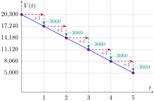
A company purchased a computer system for $\$20300\text{.}$ The company accountant decided to depreciate the item over 5 years of its “useful life” for tax purposes. The depreciated value of the system, $V(t)\text{,}$ in dollars, reported to the IRS $t$ years after the purchase (the so-called “carrying value”) is given by:

🔗

$t$ (years after purchase)	$0$	$1$	$2$	$3$	$4$	$5$
$V(t)$ (dollars)	$20300$	$17240$	$14180$	$11120$	$8060$	$5000$

What is the amount of depreciation over each of the five years?
🔗

🔗
What is an appropriate formula for the carrying value $V(t)\text{?}$
🔗

🔗

🔗

Solution.

We begin by calculating the change in depreciated value each year:
🔗

\begin{align*} \Delta V \amp\;=\; 17240-20300 \amp \;=\; -3060\\ \Delta V \amp\;=\; 14180-17240 \amp \;=\; -3060\\ \Delta V \amp\;=\; 11120-14180 \amp \;=\; -3060\\ \Delta V \amp\;=\; 8060-11120 \amp \;=\; -3060\\ \Delta V \amp\;=\; 5000-8060 \amp \;=\; -3060 \end{align*}

🔗

From the above, we conclude that the computer system depreciates by $\$3060$ each of the five years.
🔗

🔗
Since equal changes of $\Delta t=1$ in $t$ correspond to equal changes $\Delta V=-3060$ in the depreciated value of the computer system, $V(t)$ can be modeled by a linear function with formula:

\begin{equation*} V(t)=-3060t+20300. \end{equation*}

🔗

🔗

🔗

The depreciation method used by the accountant in Example 2.3.3 is called “straight-line depreciation”. The 5 years of useful life is prescribed by the IRS for each type of asset. Information about how the value at the end of the asset’s useful life, called the “salvage value”, is prescribed can be found in accounting books.

🔗

In the straight-line depreciation method, the fixed annual depreciation amount is calculated by taking the difference between the purchase cost and the salvage value and dividing by the number of years of useful life of the asset. For the computer system from Example 2.3.3, this calculation results in

\begin{equation*} \frac{\text{purchase cost} - \text{ salvage cost}}{\text{years of useful life}}=\frac{20300-5000}{5}=3060. \end{equation*}

🔗

The computer system is depreciating by $\$3060$ each year, so the slope of the associated line is $-3060\text{.}$ The graph of the depreciated value $V(t)$ for $0\leq t\leq 5$ is the straight line shown below.

🔗

$A short description.$

Exercises Exercises

1.

Decide if each table could represent a linear function and explain your reasoning. For each table that could represent a linear function, find a formula that matches the data given in the table.

🔗

$x$ $0$ $1$ $2$ $3$

$y$ $12.6$ $9.3$ $6.0$ $2.7$

🔗
$t$ $-1$ $1$ $3$ $5$

$f(t)$ $0.1$ $0.4$ $0.7$ $1.0$

🔗
$n$ $0$ $1.5$ $3$ $4.5$ $6$

$g(n)$ $12$ $18$ $12$ $6$ $12$

🔗
$t$ $0$ $2$ $4$ $6$ $8$

$h(t)$ $6.4$ $1.6$ $0.4$ $0.1$ $0.025$

🔗
$z$ $-2$ $1$ $4$ $7$

$w(z)$ $6$ $4.8$ $3.6$ $2.4$

🔗

Solution.

linear with equation $y=-3.3x+12.6$

🔗
linear with equation $f(t)=0.15t+0.25$

🔗
not linear

🔗
not linear

🔗
linear with equation $w(z)=-0.4z+5.2$

🔗

🔗

2.

The table below shows for each temperature $F$ in degrees Fahrenheit the corresponding approximate temperature $C$ in degrees Celsius. Is it appropriate to model $C$ by a linear function of $F\text{?}$ If it is, find a formula for $C$ as a function of $F\text{.}$

🔗

$F$ (degrees Fahrenheit)	$32$	$42$	$52$	$62$
$C$ (degrees Celsius)	$0$	$5.55$	$11.12$	$16.67$

Solution.

approximately linear with approximate equation $C=0.555F-17.76$

🔗

3.

The height of a human individual can be estimated by the length of the femur, as shown for males in the following table.

🔗

$L$ (length of femur in cm)	$42$	$45$	$48$	$51$
$H$ (height of human male in cm)	$162.97$	$169.93$	$176.89$	$183.85$

Use the information in this table to find a possible formula for the height of a human male $H$ as a function of his femur length $L\text{.}$

🔗
What would the approximate height of a human male with femur length 46 cm be?

🔗
Fernando is 175.4 cm tall. What would you expect the approximate length of his femur to be?

🔗

Solution.

$\displaystyle H=2.32L+65.53$

🔗
$172.25$ cm

🔗
approximately 47.36 cm

🔗

🔗

4.

The weight of water above a scuba diver as well as the air above the diver exerts pressure on their bodies. The pressure the diver experiences at sea level is $14.7$ PSI (pounds per square inch), and this pressure increases by $0.4$ PSI per each foot of depth.

🔗

Write a linear equation expressing the pressure $P$ on a diver at a depth of $d$ feet below sea level.

🔗
The deepest a recreational scuba diver typically dives is $130$ feet. What is the pressure on a diver at this depth?

🔗

Solution.

$\displaystyle P=0.4d+14.7$

🔗
$66.7$ PSI

🔗

🔗

5.

A hiker is at a trailhead about to climb a mountain. The temperature at the trailhead is $65^{\circ}$F. According to the standard atmosphere model

https://www.grc.nasa.gov/WWW/K-12/airplane/atmos.html, accessed: 6/25/20

the temperature drops by $0.00356^{\circ}$F per each 1 foot increase in altitude. Let $T=T(h)$ be the temperature, in $^{\circ}$F, $h$ feet above the hiker.

🔗

Write a formula for the function $T(h)\text{.}$

🔗
Find the temperature at the mountaintop that is $6210$ feet above the hiker.

🔗
Is the function $T(h)$ increasing or decreasing?

🔗

Solution.

$\displaystyle T(h)=-0.00356h+65$

🔗
$42.89$ $^\circ$ F

🔗
The function $T(h)$ is decreasing.

🔗

🔗

6.

A man goes to a gym to exercise. After $t$ minutes on a treadmill, his pulse (heart rate), $H\text{,}$ in beats per minute, is:

🔗

$t$ (minutes)	$0$	$3$	$6$	$9$	$12$	$15$
$H$ (bpm)	$85$	$87$	$89$	$91$	$93$	$95$

Is it appropriate to model $H(t)$ by a linear function? If yes, find a formula for $H(t)\text{.}$

🔗
If the function $H(t)$ can be modeled by a linear function, give units for the slope and the vertical intercept of $H(t)\text{.}$ Then explain their meaning in practical terms.

🔗

Solution.

Linear; formula $H(t)=\frac{2}{3}t+85$

🔗
The slope is $\frac{2}{3}$ bpm per minute; the practical meaning of the slope is that the man’s bpm is increasing at a rate of $\frac{2}{3}$ bpm per minute. The vertical intercept is $85$ bpm; the practical meaning of the vertical intercept is that the man’s resting heart rate (heart rate when performing no exercise on the treadmill) is $85$ bpm.
🔗

🔗

🔗

Prev Top Next

\(t\) (hours)	\(0\)	\(6\)	\(12\)	\(18\)	\(24\)	\(30\)	\(36\)	\(42\)	\(48\)
\(W(t)\) (grams)	\(7.00\)	\(7.45\)	\(7.90\)	\(8.35\)	\(8.80\)	\(9.25\)	\(9.70\)	\(10.15\)	\(10.60\)

\(t\)	\(2\)	\(4\)	\(6\)	\(8\)	\(10\)	\(12\)
\(f(t)\)	\(6.0\)	\(4.6\)	\(3.2\)	\(1.8\)	\(0.4\)	\(-1.0\)

\(x\)	\(0\)	\(3\)	\(6\)	\(9\)	\(12\)	\(15\)
\(g(x)\)	\(6\)	\(7.5\)	\(9.25\)	\(11.5\)	\(15.5\)	\(20\)

\(x\)	\(0\)	\(1\)	\(2\)	\(3\)	\(4\)	\(5\)
\(h(x)\)	\(3\)	\(4.5\)	\(6\)	\(7.5\)	\(9\)	\(10.5\)

\(t\) (years after purchase)	\(0\)	\(1\)	\(2\)	\(3\)	\(4\)	\(5\)
\(V(t)\) (dollars)	\(20300\)	\(17240\)	\(14180\)	\(11120\)	\(8060\)	\(5000\)

\(t\)	\(-1\)	\(1\)	\(3\)	\(5\)
\(f(t)\)	\(0.1\)	\(0.4\)	\(0.7\)	\(1.0\)

\(n\)	\(0\)	\(1.5\)	\(3\)	\(4.5\)	\(6\)
\(g(n)\)	\(12\)	\(18\)	\(12\)	\(6\)	\(12\)

\(z\)	\(-2\)	\(1\)	\(4\)	\(7\)
\(w(z)\)	\(6\)	\(4.8\)	\(3.6\)	\(2.4\)

\(F\) (degrees Fahrenheit)	\(32\)	\(42\)	\(52\)	\(62\)
\(C\) (degrees Celsius)	\(0\)	\(5.55\)	\(11.12\)	\(16.67\)

\(L\) (length of femur in cm)	\(42\)	\(45\)	\(48\)	\(51\)
\(H\) (height of human male in cm)	\(162.97\)	\(169.93\)	\(176.89\)	\(183.85\)

\(t\) (minutes)	\(0\)	\(3\)	\(6\)	\(9\)	\(12\)	\(15\)
\(H\) (bpm)	\(85\)	\(87\)	\(89\)	\(91\)	\(93\)	\(95\)

Section 2.3 Modeling and Numerically Given Functions

Objectives

Example 2.3.1.

Example 2.3.2.

By the way...

Example 2.3.3.

Exercises Exercises

1.

2.

3.

4.

5.

6.