In the previous section, we saw that if a function is given algebraically—by a formula—we can easily create a table of values for that function. That table of values can then be used to sketch the graph of the function, which in turn provides a visual representation of the function that can allow us to see behavior that may not be readily apparent from the formula alone.
When we study a real-life process, which inevitably involves a function of some kind, we rarely begin with a formula for a function that represents—or models—the process. Typically, we take measurements and collect and tabulate numerical data for the process we are studying. We then try to find a formula for a function that “fits” the numerical information we collected. That is, we start with a table of values and then try to find a formula for a function, not the other way around.
Finding a mathematical description of a real-life process is called mathematical modeling. A function that is given by its table of values is said to be given numerically.
If you ever kept overripe bananas in your house a bit too long, you probably experienced an invasion by fruit flies. And you probably noticed how quickly the population of fruit flies in your house was increasing. It is difficult to count the number of fruit flies in a house, but it can be done in a laboratory.
Suppose that a population of fruit flies in a laboratory experiment is initially 100 flies and it begins to grow. The size of the population, \(P\text{,}\) measured in thousands of flies, is a function of the time \(t\) since the experiment began; that is, \(P=f(t)\text{.}\) Given how quickly fruit flies multiply, it is reasonable to measure \(t\) in days. The scientists conducting the experiment do not have a formula for \(f(t)\) that describes the growth of this fruit fly population and, in general, that growth (and therefore the function \(f(t)\)) depends on many factors controlled by the lab—the temperature, food provided, etc. Taking into consideration the length of the fruit fly reproductive cycle, the scientists observe the population and take measurements every 14 days. The data they collect is provided in the table below.
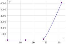
We see that \(f(t)\) is an increasing function and it increases very fast. After 56 days, the initial population of 100 flies grew to 240432.2 thousand flies; that is, 240,432,200 flies!
Can we find a formula for a function \(f(t)\) so that Table 1.3.1 is a table of values for \(f(t)\text{?}\) In other words, can we find a mathematical model for the population growth exhibited in the fruit fly experiment? It turns out that finding a formula for a function that corresponds to experimental data, even if only approximately, may be difficult. In fact, it can be impossible. A formula corresponding to Table 1.3.1can be found, as the growth of the fruit fly population is exponential. You will see how this is done when we cover exponential functions in Chapter 5.
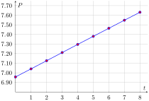
One can obtain a visual representation of a function from a numerical representation by sketching its approximate graph. The function \(f(t)\) associated with Table 1.3.1 for \(t\) between 0 and 42 is plotted below. The value at \(t=56\) is so large that it squeezes the graph vertically too much and makes it hard to read, which is why we excluded it.
On December 31, 2019 the price of ExxonMobil stock (NYSE: XOM) was changing during the day. The price of the stock each hour from 10 am to 4 pm is recorded in the table below.
Let \(E=p(t)\) be the function that gives the price of ExxonMobil stock \(t\) hours after 10 am on December 31, 2019. Rewrite Table 1.3.3 with the first row giving values of \(t\) and the second values of \(E=p(t)\text{.}\)
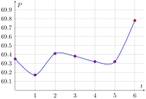
We denote by \(t\) the time, in hours, since 10 am on December 31, 2019. This means that 10 am is \(t=0\text{,}\) 11 am is \(t=1\text{,}\) 4 pm is \(t=6\text{,}\) and so on. As the function \(E=p(t)\) gives the price of ExxonMobil stock at time \(t\text{,}\) we can express \(E=p(t)\) numerically by:
The function \(p(t)\) is neither increasing nor decreasing as the graph sometimes climbs and sometimes falls as \(t\) increases. Finding a formula for the function \(p(t)\) that models fluctuations of the price of a stock does not seem simple and we will not attempt to do so.
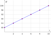
The woman’s pulse, \(H\text{,}\) is a function of time \(t\text{,}\) which, based on the table, we will measure in minutes since her treadmill workout began. We could write \(H=f(t)\) if we chose to name the associated function \(f\text{.}\) For the sake of simplicity, we often denote the dependent variable and the function by the same letter. In this case, we will instead write \(H=H(t)\text{.}\)
Can we find a formula for \(H(t)\text{?}\) We haven’t developed any specific techniques to do so yet, and hence to answer this question we can only attempt to observe patterns and make educated guesses based on common sense.
Looking at the data in Table 1.3.6, we can see that the woman’s pulse \(H\) increases as time \(t\) increases, which we might expect based on our own experience with exercise. How does \(H\) increase? The initial value of \(H\)—\(H(0)\) in function notation—is \(80\text{.}\) During the first two minutes from \(t=0\) to \(t=2\text{,}\) her pulse increases by \(4\) bpm from \(80\) to \(84\text{.}\) During the next two minutes from \(t=2\) to \(t=4\text{,}\) her pulse increases again by \(4\) bpm from \(84\) to \(88\text{.}\) Looking at each of the remaining two-minute intervals, we see that her pulse increases by \(4\) bpm every two minutes: \(88\) to \(92\text{,}\)\(92\) to \(96\text{,}\) and \(96\) to \(100\text{.}\)
As we attempt to find a possible formula for \(H(t)\text{,}\) we observe that if her pulse is increasing by \(4\) bpm every two minutes, we could perhaps think of this as \(2\) bpm every \(1\) minute instead. So her pulse starts at an initial value of \(80\) bpm and then we add \(2\) bpm for every one-minute change in \(t\text{.}\) The formula that reflects that is:
\begin{equation*}
H(t)=80+2t.
\end{equation*}
Let’s check if the values of \(H(t)\) reflect the data in Table 1.3.6:
Note that the formula \(H(t)=80+2t\) gives a possible formula for \(H(t)\text{.}\) It is entirely possible that the woman’s actual heart rate at time \(t=1.5\) minutes does not match what the formula \(H(t)=80+2t\) suggests it should be. We have no way of knowing, as the table does not tell us anything about the values of \(H(t)\) at any times other than \(t=0,2,4,6,8,10\) minutes.
We notice that the values of \(f(x)\) for each \(x\) given in the table are negative and have the magnitude equal to \(x^{2}\text{.}\) Hence, a possible function represented by Table 1.3.8 is \(f(x)=-x^{2}\text{.}\) We can easily check that \(f(x)=-x^{2}\) works by substituting \(x=0,1,2,3,4,5\) into \(f(x)\) and calculating the corresponding values. Those are indeed \(0,-1,-4,-9,-16,\) and \(-25\text{,}\) respectively.
At \(x=0\text{,}\)\(g(0)=80\text{.}\) Then, as \(x\) increases, \(g(x)\) decreases in a very regular fashion: for each increase of 1 in \(x\text{,}\)\(g(x)\) decreases by 2. A formula that gives exactly such behavior is:
\begin{equation*}
g(x)=80-2x.
\end{equation*}
We can verify that this function produces the values in Table 1.3.9:
For now, we can only try to observe patterns and “guess” formulas for numerically given functions. As we study various families of functions, we will develop more systematic methods for finding formulas of functions given numerically.
A driver of a Volkswagen Passat fills up his gas tank and starts a highway trip to a faraway city. Let \(G\text{,}\) in gallons, be the amount of gas left in the tank after driving \(d\) miles. Fill in the missing numbers and find the gas mileage of the VW Passat; that is, the number of miles the SUV gets per gallon.
The information in the table can be rewritten so that the population, \(P\text{,}\) in billions, is a function of the number of years, \(t\text{,}\) since 2010. This rewriting has been partially completed for you. Fill in the missing values.
Is the amount of power required for the dragon to carry the knight increasing or decreasing as its speed increases? Explain how you arrive at your conclusion from the data in the table.
Is the amount of power required for the dragon to carry the knight changing faster and faster or slower and slower as its speed increases? Explain how you arrive at your conclusion from the data in the table.
The amount of power required for the dragon to carry the knight is increasing as the dragon’s speed increases. This is evident from the table since the values associated with the power required increase as the speed increases.
The amount of power required for the dragon to carry the knight is increasing faster and faster as the dragon’s speed increases. This is evident from the table since each time the speed increases by 10 miles per hour starting at 60 miles per hour, the power required to carry the knight increases by more and more.
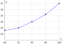
Is the amount of power required for the dragon to carry the knight increasing or decreasing as its speed increases? Explain how you arrive at your conclusion from the graph.
Is the amount of power required for the dragon to carry the knight changing faster and faster or slower and slower as its speed increases? Explain how you arrive at your conclusion from the graph.
The amount of power required for the dragon to carry the knight is increasing as the dragon’s speed increases. This is evident from the graph since it climbs over the interval \(60\leq x \leq 100\text{.}\)
The amount of power required for the dragon to carry the knight is increasing faster and faster as the dragon’s speed increases. This is evident from the graph since each time the speed increases by 10 miles per hour starting at 60 miles per hour, the graph climbs more and more quickly.
Notice that the inputs \(t\) go up by \(1\) each time. And, the outputs \(h(t)\) go down by \(2\) each time. Or, you can think of the outputs as being the inputs multiplied by \(-2\text{.}\) Therefore, \(h(t)=-2t\text{.}\) Thus \(h(5)=-10\) and \(h(6)=-12\text{.}\)
To study the population from the mathematical point of view, it is convenient to rewrite the data in terms of the independent variable \(t\) which stands for the number of years since 2010 and write the population, \(P\text{,}\) in billions, as a function \(P=P(t)\) of years since 2010. Based on the table above, fill in the missing values:
A driver of an SUV fills up his gas tank and starts a highway trip to a faraway city. Let \(G\text{,}\) in gallons, be the amount of gas left in the tank after driving \(d\) miles. Of course \(G\) is a function of \(d\text{;}\) that is, \(G=G(d)\text{.}\) Here is partial data about the function:
Except for the last column when \(d=510\text{,}\) note that the miles \(d\) go up by \(60\) each time, and the gallons \(G(d)\) go down by \(2\) each time. Using these rules, the completed table is given above. Therefore, the car can drive \(510\) miles using \(17\) gallons of gas. Thus, the gas mileage is